Maryland's Largest School District
Videos:
In this unit, your student will be learning about analyzing data. Statistics can help us recognize trends in what is typical, as well as how far from typical we can expect to go. For example, imagine you discover that one of your student’s childhood toys is actually worth a lot of money from toy collectors. What is a good price for the toy, and where should you sell it? You find two sites where you could auction the toy: one is a site for toy collectors and one is a general online site for selling items. After doing some research, you come across two histograms showing the price when other people sold this toy, as well as some statistics about the prices.
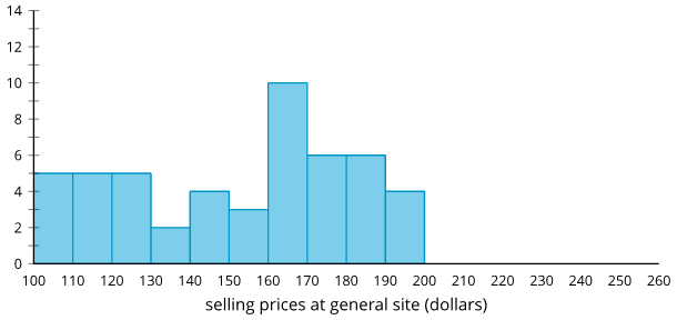
General site:
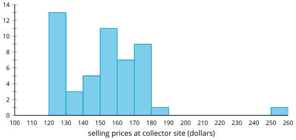
Collector site:
The first thing you may notice is that one of the toys on the collector site sold for between 250 & 260. An extremely high value like this can be called an “outlier” and should be investigated to understand why it is so different. In this case, the toy was in its original box and signed by the toy maker. Although we don’t usually like to throw out data, it doesn’t make sense to include that value when comparing to our toy, so you might take out that value to get new statistics. This changes the average price at the collector site to 150.51 and the standard deviation to 18.65. Next, you might notice that the prices for the general site are more spread out than at the collector site. This spread can be represented with a value called the “standard deviation.” The general site has a much larger standard deviation, indicating its prices are more spread out. For you, that means you are more likely to sell our toy near the average price on the collector site while the general site is more likely to sell significantly higher or lower than average.
A football coach is considering adding one of two running backs to the team. Some statistics for the number of yards gained on each run for each player are given. Which player should the coach choose? Explain your reasoning. Running back A:
Running back B:
Either running back can be a good choice for the team depending on what the coach is looking for. Running back A gets more yards per run on average, but is a lot more variable (based on the standard deviation). This means Player A sometimes has really long runs and sometimes very short (or even negative) runs. Running back A will likely be more exciting to watch, but could also be frustrating when they don’t get the needed yards. Running back B gets fewer yards per run on average, but is a lot less variable (based on the standard deviation). This means that Player B is more consistent and gets close to 4 yards every play they are allowed to run. Running back B will likely be less exciting to watch, but can be relied on to get consistent gains.
IM Algebra 1 is copyright 2019 Illustrative Mathematics and licensed under the Creative Commons Attribution 4.0 International License (CC BY 4.0).